Transformers are already energy-based models. We just don't talk about them that way yet.

Every time you set temperature=0.7 on an API call, you're adjusting the Boltzmann temperature of an energy-based model. Every softmax over logits computes the Boltzmann distribution over negative-energy scores. The connection isn't a metaphor, it's the actual math.

And this connection is starting to matter. Three recent results:

1. A 55M-parameter energy-based reward model (127x smaller than typical reward models) boosts Llama 3 to 90.7% on GSM8k and 63.7% on MATH (Jiang et al., 2025).
2. Energy-Based Transformers scale 35–57% faster than standard autoregressive transformers, tested up to 120B tokens (Gladstone et al., 2025).
3. The optimal RLHF policy is literally the Boltzmann distribution over reward-weighted outputs — EBM theory gives alignment a principled foundation.

Three parts: the EBM paradigm, how to actually train them despite the intractable partition function, and where EBMs meet LLMs in practice.

The Energy-Based Model Paradigm

What Is an Energy Function?

At its core, an EBM is just a scoring function. Hand it a configuration, get back a scalar, the energy, that says how "good" or "bad" that configuration is:

$E(x;\,\theta) : \mathcal{X} \rightarrow \mathbb{R}$

Low energy means the configuration looks like real data. High energy means it doesn't. The energy function is the model.

Important distinction: a loss function is a training-time objective over parameters $\theta$. The energy function defines the model itself. Any function $f: \mathcal{X} \rightarrow \mathbb{R}$ qualifies, with no normalization constraints or factorization required.

The demo below shows this as a 3D landscape. Blue regions are low energy (good), red are high energy (bad). Training carves out valleys where real data sits, and inference means rolling a ball downhill.

The Compatibility View

More generally, given an input $x$ and a candidate answer $y$, energy measures incompatibility:

$E(x, y) \rightarrow \text{scalar}$

High energy means $x$ and $y$ don't go together. Low energy means they do. This is deliberately more general than probability: no normalization, no proper distribution required.

Practical consequence: inference becomes optimization.

$Y^* = \arg\min_Y E(Y, X)$

No sampling, no autoregressive decoding, no beam search. Just find the $Y$ that minimizes energy.

EBMs vs. Autoregressive Models

A fundamentally different paradigm from autoregressive models:

AR models are locked into left-to-right factorization, scoring one token at a time. EBMs score entire configurations at once: bidirectional, hierarchical, compositional, whatever you want.

The Boltzmann Distribution

When you do need probabilities from an energy function, the bridge is the Boltzmann distribution:

$p(x) = \frac{\exp(-E(x) / T)}{Z}$

$Z = \int \exp(-E(x) / T)\, dx \quad \text{(the partition function)}$

Why Boltzmann specifically? The maximum entropy principle: among all distributions consistent with a given average energy, Boltzmann has maximum entropy.

Temperature as a Sharpness Control

$T$ controls how peaked vs. flat the distribution is. Low $T$ concentrates mass on the lowest-energy states (deterministic). High $T$ smears it everywhere (exploratory).

Try it yourself below. Switch between energy landscapes (quadratic, double well, multi-modal) and crank the temperature up and down.

Connection to Transformer Decoding

Here's the punchline. When a transformer produces logits $z_1, z_2, \ldots, z_V$ over the vocabulary and you compute $\text{softmax}(z_i / T)$, you're treating negative logits as an energy function and computing the Boltzmann distribution at temperature $T$.

• temperature=0.3 → sharp peaks, deterministic output (low Boltzmann temperature)
• temperature=1.5 → flat distribution, "creative" output (high Boltzmann temperature)

The connection is exact, not an analogy.

The Partition Function Problem

The partition function $Z = \int \exp(-E(x))\, dx$ sums over all possible configurations. For real problems, that space is absurdly large:

• Images (256x256x3, 8-bit): $256^{256 \times 256 \times 3} \approx 10^{473{,}000}$ possible images
• Text (length 1000, vocab 50k): $50{,}000^{1000}$ possible sequences

Computing $Z$ exactly is completely intractable. This is the reason EBMs fell out of fashion, and the central challenge behind everything in Part 2.

Two-Phase Training

Despite the intractable $Z$, we can still derive the gradient of the negative log-likelihood. Starting from:

$L(\theta) = \mathbb{E}_{x \sim p}[-\log p_\theta(x)]$

Combining steps, the gradient splits into two terms:

$\nabla_\theta L(\theta) = \underbrace{\mathbb{E}_{x^+ \sim p_{\text{data}}}[\nabla_\theta E_\theta(x^+)]}_{\text{Positive Phase}} - \underbrace{\mathbb{E}_{x^- \sim p_\theta}[\nabla_\theta E_\theta(x^-)]}_{\text{Negative Phase}}$

The fundamental equation of EBM training. The interpretation is satisfying:

• Positive Phase: Push energy down on real data. Straightforward, just compute gradients on dataset samples.
• Negative Phase: Push energy up on model samples. Sample from $p_\theta$, raise energy there, erode misallocated probability mass.

Skip the negative phase and the model assigns low energy everywhere. It learns "real data is good" but never learns what's bad.

Watch two-phase training in action below. Energy gets pulled down at data points and pushed up everywhere else.

How to Train Your EBM

The negative phase requires sampling from $p_\theta(x) = \frac{\exp(-E_\theta(x))}{Z_\theta}$, but $Z_\theta = \int \exp(-E_\theta(x))\,dx$ is intractable. Three approaches, each with different tradeoffs.

Approach 1: Markov Chain Monte Carlo

The Idea

We can't sample from $p_\theta$ exactly, but we can approximate it by running a Markov chain that converges to $p_\theta$ in the limit. Here's a key insight: the score $\nabla_x \log p_\theta(x) = -\nabla_x E_\theta(x)$ doesn't need $Z$, so gradient-based MCMC works.

Langevin Dynamics

Start from a random point, iteratively follow the energy gradient with noise:

$x_{k+1} = x_k - \frac{\varepsilon^2}{2} \nabla_x E_\theta(x_k) + \varepsilon \, z_k, \quad z_k \sim \mathcal{N}(0, I)$

Three components:

• $x_k$ — current position in configuration space
• $\frac{\varepsilon^2}{2} \nabla_x E_\theta(x_k)$ — move toward lower energy (signal)
• $\varepsilon \, z_k$ — stochastic exploration (noise)

When $\varepsilon \to 0$ and $K \to \infty$, $x_K$ distributes as $p_\theta(x)$ under regularity conditions. Plug Langevin samples into the two-phase gradient:

$\nabla_\theta L(\theta) \approx \frac{1}{N}\sum_{i} \nabla_\theta E_\theta(x_i^+) - \frac{1}{M}\sum_{j} \nabla_\theta E_\theta(x_j^-)$

where $x_i^+$ are data samples (minibatch) and $x_j^-$ are Langevin samples from the model.

The Problem with MCMC

Langevin dynamics can take a very long time to converge, especially with multiple modes separated by high-energy barriers. The chain gets trapped in one mode, negative samples only represent that region, and the other modes go untouched. 10,000 Langevin steps per sample, samples needed for every gradient update during training. The whole thing is prohibitively slow.

Contrastive Divergence

Hinton (2002)'s workaround: don't run the chain to convergence. Start from a data point, run only $k$ steps:

• CD-1: One MCMC step from data. Very biased, doesn't represent true MLE, but works surprisingly well in practice.
• Persistent CD (Tieleman, 2008): Don't reset the chain between updates, carry over the state. Works because model parameters change slowly between updates.
• Replay Buffer (Du & Mordatch, 2019): Keep historical MCMC states in a buffer, randomly sample to initialize new chains.

The demo below lets you play with both modes. Langevin: white particles explore from random starts. CD: green data points spawn red negative samples that walk a fixed number of steps.

Approach 2: Score Matching

The Score Function

What if we could skip sampling entirely? The score function is the gradient of the log density w.r.t. the input:

$s(x) = \nabla_x \log p(x)$

For an EBM with $p_\theta(x) = \exp(-E_\theta(x))/Z_\theta$:

$s_\theta(x) = \nabla_x \log p_\theta(x) = \nabla_x[-E_\theta(x) - \log Z_\theta] = -\nabla_x E_\theta(x)$

Why Scores Are Enough

If two continuously differentiable log PDFs have the same first derivative everywhere and both integrate to 1, they're the same distribution. So match scores instead of probabilities:

$s_\theta(x) = s_{\text{data}}(x) \;\; \forall x \;\;\Longrightarrow\;\; p_\theta \equiv p_{\text{data}}$

Fisher Divergence

Formally, minimize the Fisher divergence between model and data scores:

$D_F(p_{\text{data}} \| p_\theta) = \frac{1}{2}\mathbb{E}_{x \sim p_{\text{data}}}\!\left[\|s_{\text{data}}(x) - s_\theta(x)\|^2\right]$

Expanding the squared norm:

$= \frac{1}{2}\mathbb{E}\!\left[\|s_\theta\|^2\right] - \mathbb{E}\!\left[s_\theta^\top s_{\text{data}}\right] + \underbrace{\frac{1}{2}\mathbb{E}\!\left[\|s_{\text{data}}\|^2\right]}_{\text{constant}}$

Problem: the cross-term contains $s_{\text{data}}(x) = \nabla_x \log p_{\text{data}}(x)$ — we don't know $p_{\text{data}}$, only have samples from it.

The Integration by Parts Trick

Hyvärinen (2005) showed the Fisher divergence can be rewritten using only the model's score and its Jacobian:

$D_F = \mathbb{E}_{x \sim p_{\text{data}}}\!\left[\frac{1}{2}\|s_\theta(x)\|^2 + \text{tr}(\nabla_x s_\theta(x))\right] + \text{const}$

The trace term acts as an implicit negative phase, penalizing high score magnitude everywhere (same contrastive role as the negative phase in MLE). But computing that trace requires second-order derivatives, $O(d)$ backward passes for dimensionality $d$. For high-dimensional data, this is brutal.

Denoising Score Matching

Vincent (2011) found a clever workaround. Don't match scores on clean data, corrupt it first: $\tilde{x} = x + \sigma\varepsilon$, where $\varepsilon \sim \mathcal{N}(0, I)$.

Since the noise kernel $q(\tilde{x}|x) = \mathcal{N}(\tilde{x};\, x,\, \sigma^2 I)$ is a known Gaussian, its score has a simple closed form:

$\nabla_{\tilde{x}} \log q(\tilde{x}|x) = -(\tilde{x} - x)/\sigma^2 = -\varepsilon/\sigma$

Match the model's score $s_\theta(\tilde{x})$ to this known target:

$J_{\text{DSM}}(\theta) = \mathbb{E}_{x \sim p_{\text{data}},\, \varepsilon \sim \mathcal{N}(0,I)}\!\left[\left\|s_\theta(x + \sigma\varepsilon) + \varepsilon/\sigma\right\|^2\right]$

No second-order derivatives, no unknown $p_{\text{data}}$. Just a regression problem: predict the noise direction from the noisy input.

Connection to Diffusion Models

Do denoising score matching at many noise levels, from pure noise down to near-zero, and you get a multi-scale score model. Sample by starting from noise and gradually denoising via Langevin dynamics at decreasing noise scales (annealed Langevin dynamics).

Approach 3: Noise Contrastive Estimation

The Idea

Forget sampling from $p_\theta$. Forget matching its score. Just train a binary classifier: did this sample come from the data or from a known noise distribution? The theoretical guarantee: an optimal classifier implicitly recovers the data density (Gutmann & Hyvärinen, 2010).

Bonus: NCE learns $Z$ as a by-product. The only method of the three that does.

NCE Setup

Two ingredients:

1. Data distribution $p_{\text{data}}$: samples from the training set
2. Noise distribution $p_{\text{noise}}(x)$: Gaussian, uniform, or (spoiler alert) the output of a pretrained autoregressive model

We need to sample from $p_{\text{noise}}$ and evaluate its density $p_{\text{noise}}(x)$ at any point. Mix the two sources with equal probability, ask the classifier: "which source?"

NCE Optimality

At convergence, the classifier's posterior matches the true one:

$\frac{\tilde{p}_\theta(x)}{\tilde{p}_\theta(x) + p_{\text{noise}}(x)} \;\approx\; \frac{p_{\text{data}}(x)}{p_{\text{data}}(x) + p_{\text{noise}}(x)}$

At optimality, $p_{\theta^*}(x) \equiv p_{\text{data}}(x)$. NCE parameterizes $\log \tilde{p}_\theta(x) = -E_\theta(x) + c$, making the log-normalizer a learnable scalar optimized jointly with $\theta$. At convergence, $c \to -\log Z_\theta$, so you get $Z$ for free.

The NCE Objective

The loss is binary cross-entropy, classifying each sample as data or noise:

$L_{\text{NCE}}(\theta) = \mathbb{E}_{x \sim p_{\text{data}}}\!\left[\log \sigma\!\left(\log \tilde{p}_\theta(x) - \log p_{\text{noise}}(x)\right)\right] + \mathbb{E}_{x \sim p_{\text{noise}}}\!\left[\log \sigma\!\left(\log p_{\text{noise}}(x) - \log \tilde{p}_\theta(x)\right)\right]$

Positive and negative phases emerge naturally from the two cross-entropy terms. $E_\theta$ gets updated so the model assigns high density to data, low density to noise.

No MCMC. No Hessian. No score functions. Just a classifier and a good noise distribution.

Why Hard Negatives Matter

The closer the noise distribution is to the real data, the harder the classifier has to work, and the better the representations:

• Easy noise (e.g., uniform): trivial to classify → model learns superficial features
• Hard noise (e.g., pretrained LM): hard to classify → model must learn deep structure

Same principle behind SimCLR, CLIP, and ELECTRA. Harder negatives, better representations. This comes back in Part 3.

Comparing Training Paradigms

Three different tricks for the same intractable $Z$: MCMC sidesteps it with sampling, score matching removes it via calculus, NCE absorbs it into a classifier.

EBMs Meet LLMs

Theory's done. How are people actually using this stuff with LLMs? The approaches range from conservative (slap an energy correction on top) to radical (replace the whole architecture).

Your Classifier Is Secretly an EBM

JEM: Joint Energy Models

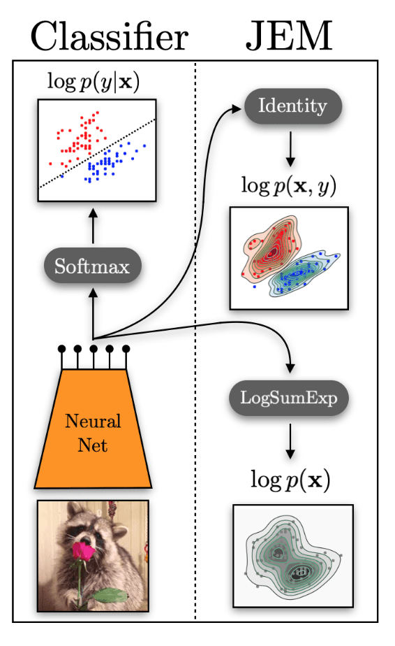
Grathwohl et al. (2020) noticed something surprising: every standard classifier with a softmax output already contains a hidden energy-based generative model.

A standard classifier computes:

$p_\theta(y \mid x) = \frac{\exp(f_\theta(x)[y])}{\sum_{y'} \exp(f_\theta(x)[y'])}$

The reinterpretation: treat logits as a joint energy function:

$p_\theta(x, y) = \frac{\exp(f_\theta(x)[y])}{Z(\theta)}, \quad E_\theta(x,y) = -f_\theta(x)[y]$

Marginalize out $y$ to get an energy over inputs:

$E_\theta(x) = -\text{LogSumExp}_y\, f_\theta(x)[y] = -\log \sum_y \exp(f_\theta(x)[y])$

Training the Joint EBM

JEM decomposes the joint log-prob:

$\log p_\theta(x, y) = \underbrace{\log p_\theta(x)}_{\text{SGLD}} + \underbrace{\log p_\theta(y \mid x)}_{\text{cross-entropy}}$

The generative term $\log p_\theta(x)$ trains via SGLD (Langevin dynamics); the discriminative term $\log p_\theta(y|x)$ uses standard cross-entropy.

Results on WideResNet + CIFAR: JEM gets better classification than discriminative-only, better generation (FID) than generative-only baselines (Glow, flow models), improved calibration, strong OOD detection via the energy score, and better adversarial robustness. Same set of logits. No extra parameters. Just a reinterpretation of what was already there.

ELECTRA and the EBM Connection

ELECTRA: Pre-Training Text Encoders as Discriminators

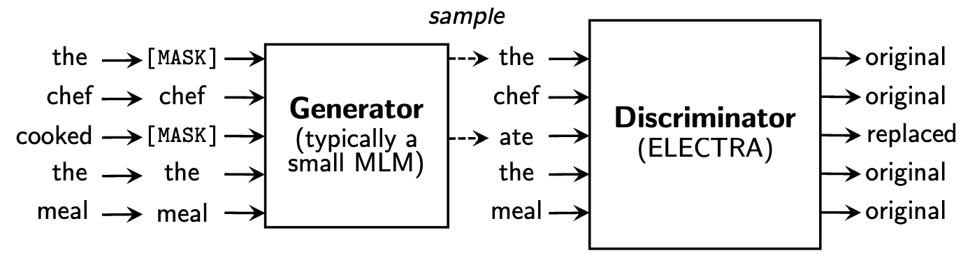
ELECTRA (Clark et al., 2020): train a small generator (MLM) to fill in masked tokens, then a larger discriminator classifies each token as original or replaced.

Why better than BERT's masked LM?

• Dense signal over all tokens (not just ~15% masked)
• No [MASK] token mismatch between pre-training and fine-tuning
• 3–7x sample efficiency over BERT

Notice anything interesting 👀? ELECTRA is NCE with the generator as the noise distribution. Data distribution = real tokens from the corpus. Noise distribution = tokens from the small MLM generator. Classifier = ELECTRA discriminator (the model we keep). The generator provides hard negatives: replaced tokens that are plausible in context, forcing the discriminator to learn deep linguistic structure.

Electric: Energy-Based Cloze Models

Electric (Clark et al., 2020) pushes ELECTRA's insight further, from binary classification to proper NCE.

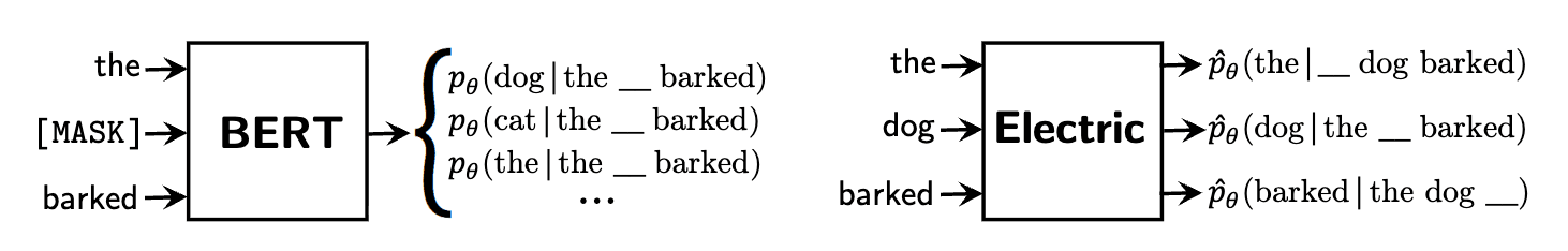
BERT predicts a distribution over the vocabulary at masked positions (learning from ~15% of tokens). Electric outputs a cloze probability for every token $\hat{p}_\theta(x_i \mid x_{\backslash i})$, i.e. how likely is this specific token in this position? Dense signal from every token, no [MASK] needed.

It uses the generator's known density to convert discriminator output into calibrated per-token pseudo-probabilities, making it a true energy-based model over token configurations. And because it models per-token cloze probabilities (not joint sequence probability), it sidesteps autoregressive factorization entirely.

Residual EBMs for Text

Deng et al. (2020) took a pragmatic approach: keep the pretrained AR model, multiply its distribution by an energy correction from a bidirectional model:

$P(x) = P_{\text{LM}}(x) \cdot \frac{\exp(-E_\theta(x))}{Z}$

AR handles fluency and local coherence (token-by-token). The bidirectional energy provides global, sequence-level quality correction. The EBM doesn't generate, it scores and corrects. Trained end-to-end via NCE.

EDLM: Energy-Based Diffusion Language Models

The Problem with Parallel Text Generation

Discrete diffusion models unmask tokens in parallel, but they predict each token independently:

$p_\theta(x_0 \mid x_t) = \prod_i p_\theta(x_0^i \mid x_t) \quad \text{(independent per token!)}$

Each denoising step predicts a clean token at every masked position conditioned only on the noisy context, with no inter-token dependencies within the same step. The more parallel you go (fewer denoising steps), the worse this factorization error gets. That's the fundamental gap between diffusion and AR quality for language.

Residual Energy Correction

Ye et al. (2024) apply residual energy correction at every denoising step:

$p_{\theta,\phi}(x_0 \mid x_t) = p_\theta(x_0 \mid x_t) \cdot \frac{\exp(-E_\phi(x_0, x_t, t))}{Z_\phi(x_t)}$

Two instantiations:

• EDLM-AR: Plug in a pretrained AR model as the energy. One AR forward pass scores a complete sequence, enabling parallel sampling from an AR model via importance weighting.
• EDLM-NCE: Train a small energy head via NCE on top of the diffusion model. Positives = clean data, negatives = the diffusion model's own predictions.

At inference, draw $k$ candidates from the diffusion model, score with energy, resample via importance weights. The correction matters most in early denoising steps (high masking ratio → worst factorization error). Applying importance sampling only for $t \in [0.8, 1.0]$ captures most of the benefit at a fraction of the cost.

The numbers: 49% generative perplexity improvement, 1.3x sampling speedup at same quality, 400k fine-tuning steps for the NCE variant. The generation uses parallel importance sampling: draw multiple candidates simultaneously and reweight by energy, not sequential rejection sampling. Published at ICLR 2025, EDLM was the first diffusion model to seriously challenge AR quality on language.

Energy-Based Transformers

Gladstone et al. (2025) go all the way. Inspired by System 2 Thinking: the entire model is an energy function that learns to verify compatibility between inputs and predictions, through unsupervised learning alone.

$E_\theta(x, \hat{y}) \rightarrow \text{scalar} \quad \text{(how compatible is prediction } \hat{y} \text{ with context } x \text{?)}$

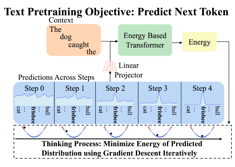
Architecture: standard Transformer++ backbone (RMSNorm, SwiGLU, RoPE) where the LM head is replaced with an energy head that outputs a single scalar instead of a distribution over the vocabulary. The prediction $\hat{y}$ lives in continuous embedding space (not discrete token IDs), which is what enables gradient-based refinement.

Training uses denoising score matching: corrupt ground-truth embeddings with Gaussian noise at varying levels, train the energy function so its gradient w.r.t. the noisy input points toward clean data. Same signal as diffusion models, but without a separate base model. The energy function IS the model.

Inference is gradient descent from random noise to a converged prediction:

$\hat{y}_{i+1} = \hat{y}_i - \alpha \cdot \nabla_{\hat{y}_i} E_\theta(x, \hat{y}_i) \quad \text{(gradient w.r.t. prediction, not parameters)}$

Each gradient step is one unit of thinking. The model is simultaneously a generator (via energy minimization) and a verifier (via the energy scalar).

Three Facets of System 2 Thinking

EBTs get three properties that standard transformers lack:

• Dynamic Compute: Iterate more on harder predictions. Same compute for "the" as "serendipitous"? Not anymore.
• Uncertainty: Energy at convergence directly quantifies confidence. Easy tokens → low energy. Hard tokens → high energy.
• Verification: Best-of-N sampling without a separate reward model. The energy IS the verifier.

All three emerge from unsupervised pretraining. No RL, no verifiable rewards.

Scaling Results

EBTs are the first architecture to out-scale Transformer++ across multiple axes simultaneously, tested on both text and vision:

• 35% faster scaling on data
• 28% faster scaling on batch size
• 57% faster scaling on depth
• 29% inference improvement via thinking

On image denoising, EBTs beat Diffusion Transformers with fewer forward passes. On language, despite slightly worse pretraining perplexity, EBTs win on most downstream tasks. Verification generalizes better than raw prediction.

Thinking at Inference Time

EBTs improve with more forward passes. Standard Transformer++ can't. Two key findings:

• OOD thinking boost: The more out-of-distribution the data, the more thinking helps. Just like humans engage deliberate reasoning for unfamiliar problems.
• Thinking scales with training: More training data → more benefit from self-verification (4–8% → 10–14%). Extrapolation to Llama-3 scale suggests potentially massive gains.

Further Reading

Three more recent papers worth knowing about:

ARMs are Secretly EBMs (Blondel et al., 2025)

Google DeepMind establishes an explicit bijection between ARMs and EBMs in function space, starting from the chain rule of probability. This bijection corresponds to a special case of the soft Bellman equation in max-entropy RL, giving a formal justification for why next-token predictors can plan ahead despite sequential prediction. They also derive equivalences for supervised learning and error bounds for distilling EBMs into ARMs. The takeaway: AR vs. EBM is less about architecture, more about how you train and decode.

CALM: Continuous Autoregressive Language Models (Phan et al., 2025)

Google DeepMind replaces the discrete softmax head with an energy-based generative head that predicts continuous vectors. A lightweight residual MLP predicts $K$ tokens at once via energy minimization instead of categorical sampling, bridging AR and energy-based approaches.

EORM: Energy Outcome Reward Model (Jiang et al., 2025)

UCLA builds a 55M-parameter energy-based reward model that ranks Chain-of-Thought solutions, 127x smaller than typical reward models (often 7B+). Base LLM generates $N$ CoT solutions, EORM scores each with its energy, and you pick the lowest. Best-of-N reranking with negligible overhead. Trained with simple outcome labels (was the final answer correct?), not expensive step-level process supervision.

Results: Llama 3 8B → 90.7% on GSM8k and 63.7% on MATH. It generalizes to OOD problems and unseen models, capturing reasoning principles rather than memorized patterns. The "EBM as verifier" pattern at its most practical: a tiny energy model giving outsized improvements to a much larger generator.

The Spectrum of Energy-Based LLMs

Where do all these approaches sit?

• Conservative — EBM as correction layer: JEM, Electric, Residual EBMs, EDLM, EORM. Keep your existing models, add energy scoring on top. Already works at scale.
• Radical — EBM as the whole model: EBTs, CALM. The transformer IS the energy function. Theoretically cleaner, remarkable scaling, built-in verification.
• Unifying — ARMs $\equiv$ EBMs: Blondel et al. show every AR model has an equivalent EBM via the chain rule. The real distinction is training and decoding, not architecture.

Key Takeaways

1. Verification scales better than generation. EBTs scale 35–57% faster than feed-forward predictors. Scoring is easier than producing (P vs NP intuition applied to neural nets).

2. Test-time compute has a principled framework. Each gradient step is a thinking step, energy measures confidence, convergence gives a stopping criterion. No ad-hoc prompting tricks.

3. Composition is the killer feature. Energy functions add. Want fluency + factuality? Add their energies. Modular, tunable, no retraining.

4. The open question is scale. No known EBM operates at GPT-4 scale. EBT experiments top out at 800M parameters. The training and sampling challenges that plagued classical EBMs may resurface at frontier model sizes: mode collapse, mixing time, all of it.

References

• [1] Song, Y. & Kingma, D.P. (2021). How to Train Your Energy-Based Models. arXiv preprint arXiv:2101.03288. — Tutorial and survey on EBM training methods (MCMC, score matching, NCE).

• [2] Grathwohl, W., Wang, K.C., Jacobsen, J.H., Duvenaud, D., Norouzi, M., & Swersky, K. (2020). Your Classifier is Secretly an Energy Based Model and You Should Treat it Like One. ICLR 2020. — Introduced Joint Energy Models (JEM).

• [3] Clark, K., Luong, M.T., Le, Q.V., & Manning, C.D. (2020). ELECTRA: Pre-training Text Encoders as Discriminators Rather Than Generators. ICLR 2020. — Replaced masked language modeling with replaced token detection.

• [4] Clark, K., Luong, M.T., Le, Q.V., & Manning, C.D. (2020). Pre-Training Transformers as Energy-Based Cloze Models. EMNLP 2020. — Electric: energy-based per-token cloze scoring via NCE.

• [5] Deng, Y., Bakhtin, A., Ott, M., Szlam, A., & Ranzato, M. (2020). Residual Energy-Based Models for Text Generation. ICLR 2020. — Combining AR language models with bidirectional energy corrections.

• [6] Ye, J., Xu, M., Geffner, T., Kreis, K., & colleagues. (2024). Energy-Based Diffusion Language Models for Text Generation. ICLR 2025. — Residual EBM correction for discrete diffusion models.

• [7] Gladstone, A. & colleagues. (2025). Energy-Based Transformers are Scalable Learners and Thinkers. arXiv preprint arXiv:2507.02092. — Full energy-based transformer architecture with System 2 thinking.

• [8] Blondel, M., Sander, M.E., Vivier-Ardisson, D., Liu, L., & Roulet, V. (2025). Autoregressive Language Models are Secretly Energy-Based Models. Google DeepMind. — Exact bijection between ARMs and EBMs via the soft Bellman equation.

• [9] Phan, H., Tschannen, M., Grathwohl, W. & colleagues. (2025). Continuous Autoregressive Language Models (CALM). Google DeepMind. — Energy-based continuous head for multi-token prediction.

• [10] Jiang, Y., Luo, H., Pang, R.Y. & colleagues. (2025). Learning to Rank Chain-of-Thought: Energy Outcome Reward Model (EORM). UCLA. — 55M-parameter energy-based reward model for CoT ranking.

• [11] Gutmann, M.U. & Hyvärinen, A. (2010). Noise-Contrastive Estimation: A New Estimation Principle for Unnormalized Statistical Models. AISTATS 2010. — Foundational paper on NCE.

• [12] Hyvärinen, A. (2005). Estimation of Non-Normalized Statistical Models by Score Matching. JMLR, 6, 695–709. — Introduced score matching for unnormalized models.

• [13] Vincent, P. (2011). A Connection Between Score Matching and Denoising Autoencoders. Neural Computation, 23(7). — Denoising score matching.

• [14] Hinton, G.E. (2002). Training Products of Experts by Minimizing Contrastive Divergence. Neural Computation, 14(8), 1771–1800. — Introduced contrastive divergence for EBM training.

• [15] Song, Y. & Ermon, S. (2019). Generative Modeling by Estimating Gradients of the Data Distribution. NeurIPS 2019. — Score-based generative models via annealed Langevin dynamics.

• [16] Ho, J., Jain, A., & Abbeel, P. (2020). Denoising Diffusion Probabilistic Models. NeurIPS 2020. — DDPM: the probabilistic lens on denoising score matching.